Unlocking Financial Futures: The Evolution of Wealth Management

Wealth management Introduction

Wealth management is the analysis of a person’s current financial situation and financial goals to create an efficient investment strategy which will grow an owner’s assets while protecting it. Market conditions remain unpredictable, and the future is inherently uncertain. Historical data indicates that, over a 20-year investment horizon, stocks have generated annual total returns spanning from 2% to 18%.

A diligent wealth management plan involves selecting investment strategies with diversified portfolios which generate consistent returns with low volatility regardless of market and economic environments by adapting the investment portfolio.

The iron law of wealth management is to grow a portfolio consistently with low volatility during bull markets and avoid bear markets.

The aim of wealth management is to accomplish the investor’s financial goals.

Financial goals range from supporting children, living comfortable lifestyle to a decent retirement.

The two critical tenets of wealth management are:

• The Investment Strategies selected should have the exclusive objective of minimizing the risk of not meeting the investor’s financial goals
• Risk is measured as the probability investor won’t meet her financial goals

A wealth management plan should consider investor’s financial goals and produce a plan based on a range of potential outcomes that yields the odds of success. The aim is to estimate the probability of achieving specific outcomes with good accuracy.

Reliable financial plans must be based on a good estimate for the portfolio’s expected average return and volatility over the next 20 years.

Wealth management experts aim to achieve the most consistent returns at the lowest possible risk.

Amateur investors on the other hand, simply look at upside returns while ignoring volatility and the potential for large capital losses which may lead to complete financial destruction.

The most important factors affecting the sustainable income investors strive to achieve are

1. Investments’ volatility
2. Sequence of returns risk
3. Inflation

High investment volatility, adverse sequence of returns and high inflation destroys your wealth and your retirement income. All three risk factors can be mitigated by selecting the appropriate investment strategies.

Compounding leads to Wealth Creation

To build your wealth in a short time period requires huge risks and the odds of succeeding are minimal. Most successful investors build their wealth gradually, by selecting investments which generate good returns with low risk. Your partner in building wealth is compound interest.

“Compound interest is the eighth wonder of the world.” – Albert Einstein

Compound interest is interest calculated on the initial principal and on the accumulated interest of previous periods of a deposit.  Compound interest can be thought of as “interest on interest”.

Click to Discover the power of Compounding

Compounding needs two prerequisites to work:

• Investing for long periods of time
• Never lose big amounts of money

If you invest $10,000 at 20 with a 10% yearly average rate of return in 45 years you will have $728,904. The reason is that in first year your $10K would become $11K, while during second year your $11K would grow up by 10% and you will earn interest on the principal ($10K) and the interest ($1K) of the previous year. Additionally, If you save $10,000 every year for 45 years, then you will end up with $6,526,425.

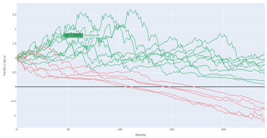
When to Stay out of the Markets

The most important investment decision is when to stay out of the markets that is hold mostly cash or other safe investments like low-risk government bonds. The reason is it is very difficult to recover from big losses during bear markets (the US Stock Market lost 38% on average).

Tip: A 50% loss requires a 100% gain to get back to even.

In the example below, experiencing three big annual losses adversely affected compounding and as a result the end value of the portfolio. More specifically, an investment of $10,000 grew to $1,8 million after 40 years instead of $24 million because of three 50% losses experienced in years 12, 24 and 36.

The reason is that any funds lost from a portfolio during a bear market could not be reinvested to help the portfolio recover during market recovery.

Portfolio Volatility

In the world of investments, achieving growth involves accepting a certain level of risk. To potentially increase your savings over an extended period, you must be prepared to endure short-term losses along the way.

The value of an investment strategy is measured in terms of how much growth it generates per unit of risk endured to generate that growth. If the expected payoffs from two investments are equal, most investors would choose the option with lower risk.

The Sharpe Ratio of any investment highlights how much return you are getting for every unit of risk you are taking. The best investment strategies have the highest sharpe ratio possible.

Portfolio Volatility is the most important factor defining your retirement income

The volatility of an investment is the most important thing defining its growth. High volatility destroys an individual’s investment portfolio and as a result his future retirement income.

Investment volatility risk is mitigated by investing in low volatility with consistent returns investments.

Assume you had to choose between two investment portfolios with the historical return performance displayed above. Although portfolio 2 has a higher ending value than portfolio 1, it has a much higher volatility and drawdown than portfolio 1. As a result, portfolio 1 sharpe ratio is 3 times higher than portfolio 2 sharpe ratio and hence portfolio 1 is preferred.

In the example above, during the second half of 2013, portfolio 2 dropped from $160,000 to $105,000 losing 35% of its value. On the other hand, portfolio 1 biggest drawdown occurred in end of 2013 losing just 4.5% of its value.

Example 2:

The compound annual growth rate of portfolio 1 is 3.9% having lost almost one fourth versus CAGR of portfolio 2. The reason is that big drops in an investment’s hurt the compound growth of the portfolio. In year 3 portfolio’s 1 value falls from $1102 to $882 and it’s very difficult for the portfolio to recover the loss as seen on the chart.

Sequence of Returns Risk

Sequence risk is the risk of receiving negative returns early or late in a period of withdrawals or savings from an individual’s investments. Sequence risk is mitigated by investing in low-volatility with consistent returns investments.

There are 2 types of sequence risk.

Saver’s Sequence risk is the risk an individual faces of losing wealth by receiving negative returns late during the period he saves to build his wealth.

Retiree’s sequence risk is the risk an individual faces of losing wealth by receiving negative returns early during a period when withdrawals are made to sustain his retirement income.

Sequence of returns for savers risk

A portfolio is build by accumulative savings gradually. However, young investors earn small amounts hence cannot make significant lump-sum investments. The majority of savings occurs in the final years before retirement. Most specifically, over 70% of total savings occur in final 10 years before retirement.

Hence, it’s very important not to have high volatility and risk of losses in the later stages before retirement, whereas young investors can take higher risks.

Example

There are 2 portfolios of a saver who annually contributes $1000 to both portfolios. Both portfolios have the same average return (4%) but different sequence of returns. Portfolio 1 experiences big losses during early years while portfolio 2 experiences the same losses late in portfolio’s life. As a result, portfolio 1 ends up after 10 years at $28231 versus portfolio 2 which ends up at $21846 having gained 29% versus portfolio 2.

The compound growth rate (definition: compound annual growth rate (CAGR) is the mean annual growth rate of an investment over a specified period of time) of portfolio 1 is 10.9% having gained almost one fourth versus CAGR of portfolio 2.

The reason is that losing 20% of $11000 (early stages of portfolio) hurts the portfolio much less than losing 20% of $27000 (late stages of portfolio).

Sequence of returns for retirees

“During the initial years of retirement, the portfolio size is comparatively substantial when compared to the annual withdrawal amounts. On the other hand, in the latter stages of retirement, after numerous years of drawing down income, the portfolio size diminishes in relation to these withdrawals.

Hence, it’s very important to have consistent returns with no losses in the early years of the retirement process.

When an extended period of subpar returns occurs early in retirement, retirees may deplete their funds entirely before reaching the midpoint of their expected lifespan.

A sequence of returns Example

There are 2 portfolios of a saver who annually withdraw $1000 from both portfolios. Both portfolios have the same average return (4%) but different sequence of returns. Portfolio 1 experiences big losses during early years while portfolio 2 experiences the same losses late in portfolio’s life. As a result, portfolio 1 ends up after 10 years at $11281 versus portfolio 2 which ends up at $17666 having gained 36% versus portfolio 2.

The compound growth rate (definition: compound annual growth rate (CAGR) is the mean annual growth rate of an investment over a specified period of time) of portfolio 1 is -5.6% having lost almost 5 times what portfolio 2 has lost.

The reason is that big drops in a portfolio’s early life hurts its compound growth. In year 1 portfolio’s 1 value falls from $20000 to $15000 and it’s very difficult for the portfolio to recover the loss during year 3-9 where 5% annual returns are generated.

Safe withdrawal rate

Retired Investors care about their safe withdrawal rate (SWR). Safe Withdrawal Rate is simply the rate that you can withdraw from your portfolio every year that ensures you have a high probability of never running out of money.

A typical SWR is 4% per year (inflation-adjusted) which according is often recommended for 30-year retirements. A couple who needs $100,000 pretax and after inflation per year to fund their lifestyle with a 4% SWR means that they would need $2,500,000 in savings.

SWR is affected by the years of retirement (affected by 1. Age of retirement and 2. living longer than expected risk) and poor investment returns generated over the investment horizon and inflation.

Every asset allocation, even 100% US Treasuries bonds has supported a 3% SWR adjusted for inflation. However, current interest rates of 1.5-1.8% are lower than they have been historically. Therefore, investors with 100% bond positions are unlikely to retire successfully with 3% SWR.

For retirees having an SWR of 3.5% to 5.5% the optimal mix historically has been stocks/bonds is 70/30.

However, the calculations above are based on historical information. Given however, current market valuations (Shiller PE), dividend yields and current interest rates quantitative models (Pfau 2013) suggest SWRs in the range of 2%.

Building a Wealth Management Strategy

The aim is to build an investment strategy for stability, growth and maximum returns.

Traditional portfolio management has proved insufficient in helping investors grow their wealth while protecting it during recessions and bear markets.

The solution is to build a flexible portfolio management framework which will adapt to economic and market conditions.

Darwin: It is not the strongest of the species that survives, nor the most intelligent. It is the one that is the most adaptable to change.

 Before exploring the adaptive method let’s have a look at the performance of static portfolio management solutions.

Building the adaptive Portfolio

The best approaches to investing is creating a diversified portfolio of assets which are uncorrelated during all market and economic environments. To do that we must firstly understand the behavior of each asset class in the portfolio.

The four economic environments

There are 4 economic environments based on economic growth and inflationary conditions.

Financial assets are affected by economic growth and inflation expectations. The performance of each financial asset for each economic environment is explained below.

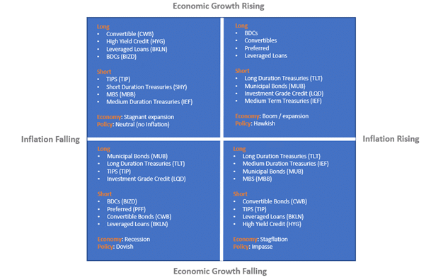
• Inflation boom: Accelerating Economic growth with Rising inflation

The best performers are emerging market stocks, international real estate, emerging countries’ currencies, commodities, and TIPS (treasury inflation protected securities).

The worst performers are US treasury bonds and cash since they are adversely affected by rising inflation.

High global growth with rising inflation expectations lifts commodities. Many emerging economies growth is linked to commodities. When commodities rise emerging market stocks, currencies and real estate rise as well.

• Stagflation: Slowing Economic Growth with Rising Inflation

Click to check the Best & Worst Assets during Stagflation

The best asset performers protecting investors from inflation are Gold, Cash, Treasury Inflation Protected Securities, and the US Dollar.

The worst performers are long-duration treasury bonds adversely affected by rising inflation.

• Disinflation boom: Accelerating Economic growth with Slowing Inflation

The best performers are developed markets stocks, developed Real estate and US Treasury bonds.

Low inflation with moderate growth is a good environment for bonds and stocks and bad for the worst performs which are commodities and commodity related sectors.

• Deflation Bust: Slowing Economic Growth with Falling Inflation

During this environment the best asset performers are Long-Duration Treasuries and Cash. Everything else experiences big volatility and often large losses.

During crashes and economic depressions bonds rise while stocks and commodities fall. Investors during these environments look for the safety of their asset rushing into the safety of US treasury bonds and the US dollar while selling stocks and commodities.

Developed Markets Equities: Stocks in developed markets respond to decreasing inflation expectations, which result in lower discount rates. However, they exhibit a more significant reaction to economic growth, as it drives increases in corporate earnings and book values. Additionally, lower inflation leads to reduced industrial and labor input costs, thereby boosting profit margins. This trend was evident from 1981 to 2000.

Emerging markets stocks: Equities are likely to outperform when global economic growth accelerates, and there’s a simultaneous increase in inflation expectations. This phenomenon can be attributed to the fact that many emerging economies are key suppliers of commodities that experience heightened demand and price increases during a global economic upswing, driven by strong demand and rising inflation expectations. An illustrative period of such economic conditions occurred from 2003 to mid-2008

US Treasuries & Gold: Treasuries and gold exemplify assets that perform well in a deflationary downturn. In situations akin to the Great Depression, the economy contracts, GDP experiences negative growth, and prices deflate, causing cash to retain its value compared to other goods and assets. In such times, declining interest rates, especially for long-duration Treasury bonds, contribute to price appreciation. Additionally, gold has historically played a significant role during these periods, as central authorities increase money supply to combat prevailing deflationary pressures.

Diversified Asset Selection

We select a diverse set of assets. The assets selected are:

1. US Stocks: VTI
2. US 7-10 Year Treasury: IEF – Bonds rise in periods of declining inflation and/or growth
3. Emerging market stocks: EEM
4. US Real Estate: ICF – Real estate rises in a periods of rising inflation
5. Commodities: DBC – Commodities rise during periods of rising inflation and/or economic stagnation

Momentum Factor

Momentum is one of the largest market inefficiencies generating consistent returns. The fundamental reason is that humans usually choose to follow the crowd rather than act against it. This causes rising prices to attract buyers and falling prices to attract sellers. Academic research has shown momentum to be a market anomaly from the early 1800s up to the present and across nearly all asset classes.

“Cut your losses; let your profits run on” – David Ricardo, 1838

The Simple Momentum Portfolio

There are many quantitative methods to apply momentum to an asset or portfolio. Our simple Momentum portfolio applies momentum as follows:

• Each asset (VTI, IEF, EEM, ICF, DBC) holds an equal weight to the portfolio (20%).
• At the end of every week, the algorithm calculates each asset’s previous 1-month (20 trading days) return
• If the return is negative or zero, we substitute the specific asset with cash (SHY).
• If the return is positive, we keep the asset in the portfolio or we buy the asset if we do not already hold it.

The Simple momentum portfolio generated impressive results while been extremely simple. The portfolio generated three times the risk-adjusted returns of the US Stock market.

The portfolio’s average annual return was 11% when the stock market’s return was 6.4%. A 56% improvement in returns was achieved with half the US Stock market’s volatility. Moreover, the Simple Momentum portfolio lost a maximum of 12.30% during it’s worst performance while the US Stock market lost 59% which is almost 5 times more.

Balancing Risk

The goal of risk parity is to build a balanced portfolio which will generate stable annual returns with lower risk than the same portfolio with equal weight among assets.

Risk parity ensures that each asset in the portfolio contributes an equal amount of risk (volatility) to the portfolio. Each asset’s weight in the balanced portfolio is calculated based on the amount of the asset’s recent volatility as compared to the volatilities of the other portfolio’s assets.

On the other hand, the simple portfolio assigns equal weight to the portfolio’s assetsfocusing on balancing the dollar amounts invested in each asset of the portfolio.

Volatility describes the degree to which an asset’s price moves up and down. Recent volatility of an asset can be estimated by calculating the recent (trailing) 20-day standard deviation of the asset’s returns

During periods of high volatility, asset returns tend to be lower and during low volatility asset returns tend to be higher. When an asset’s volatility spikes it is usually leading to big asset losses.

Balancing Volatility Example

The aim is to build a balanced portfolio with only stocks and bonds and assign equal risk contribution to both assets. The recent volatility of stocks is 2 times (200%) the observed volatility of bonds. The appropriate allocation to each asset would be computed as follows:

Allocation to stocks x volatility of stocks = allocation to bonds x volatility of bonds

Since ratio of volatility of stocks: bonds is 2:1, the allocation would be equal 1:2 that is 1/3 stocks and 2/3 bonds

Structuring the Balanced Portfolio

The Balanced portfolio is structured as follows:

• The Portfolio consists of the following assets: US Stocks (VTI), US Bonds (IEF), Emerging Stocks (EEM), US Real Estate (ICF) and Commodities (DBC)
• At the end of every week the portfolio is structured based on the following calculations:
  • Each asset’s recent 1-month (20 trading days) return is computed
  • If the return is negative or zero, the specific asset is substituted with cash (SHY) and is allocated 20% of the portfolio’s weight otherwise the asset is kept in the portfolio
  • If the return is positive, the asset is held in the portfolio or is bought back if not already included in the portfolio
  • Each asset’s recent 1-month (20 trading days) standard deviation is compued. The risk parity formula described above is used to calculate the weights of the portfolio’s assets. The risk parity formula takes into account each individual asset’s volatility versus the volatility of the rest of portfolio’s non-cash assets.

The Risk Parity portfolio generated impressive results while been very simple. The portfolio generated four times the risk-adjusted returns of the US Stock market (Sharpe Ratio of 1.20 versus 0.31 of US Stock Market).

The portfolio’s average annual return was 8.6% when the stock market’s return was 6.4%. Most importantly, the Risk Parity portfolio lost a maximum of 7.2% during its worst performance while the US Stock market lost 59%, 8 times more! This can be viewed clearly from the lower chart above where in blue is the maximum loss of the risk parity portfolio and in orange the maximum loss incurred from the US Stock market.

Risk Parity portfolio has successfully protected its investors while offering consistent returns during the last 10 years.

Portfolio Optimization

Default risk parity assumes that all assets have a correlation of zero. In reality, assets’ correlations are dynamic and almost never zero. (show charts rolling correlations of assets)

Assets which are highly correlated in the portfolio contribute much more risk than assets that are good diversifiers.

Minimum variance optimization algorithms strive to find the perfect weights of all assets in a portfolio by estimating dynamic volatilities and correlations between portfolios’ assets. These algorithms and consequently the portfolios utilizing such methods offer flexibility and short response times to changing market conditions.

Keep in mind that a good diversified selection of portfolios’ assets is a prerequisite for such algorithms to succeed in finding the optimum balance between assets.

Portfolio Leveraging

To improve the portfolio’s performance further, portfolios’ returns can be enhanced further using dynamic methods to increase portfolio leverage when markets are calm and volatility is low. This occurs typically in the early and mid-stages of bull markets. When volatility is high which is in early stage of bear markets portfolio leverage is scaled down dynamically.

Enriching the Portfolio’s Asset Selection Further

Other assets can be included in the portfolio in order to broaden the portfolio’s spectrum monitored. In this way, returns can be boosted further while maintaining low levels of volatility.

Investment Strategies

You can access our investment strategies section to research and implement strategies of different trading styles.